How to Filter Colored Cells in Excel: Simple Instructions

If your Excel sheet looks like a bag of Skittlesred for “urgent,” yellow for “check this,” green for “approved,” and that mysterious purple someone used “just because”you’re not alone. The good news: Excel can filter by cell color, font color, and even conditional formatting icons. The better news: you don’t need to be an Excel wizard. You just need to click the right tiny arrow that Excel hides like it’s playing a game of “find me.”

This guide walks you through how to filter colored cells in Excel with clear steps, practical examples, and a few “don’t do this unless you enjoy chaos” tips. You’ll also learn what to do when Filter by Color is missing or not working, plus several workarounds for more advanced needs.

Why Filter by Color in Excel?

Filtering by color is useful when color is your visual shorthand for meaning, such as:

• Project management: red rows = blockers, yellow = waiting, green = done
• Audits and review: highlighted cells = items that changed or need verification
• Data cleanup: colored flags for duplicates, errors, or missing values
• Sales and inventory: conditional formatting icons showing trends or thresholds

Color-based filtering doesn’t replace structured data (like a “Status” column), but it’s a fast way to isolate what your eyes already understand.

Before You Start: A Quick Checklist

Filtering by color works best when your data is set up cleanly. Take 30 seconds to check these:

• One header row at the top (column names like “Customer,” “Status,” “Amount”).
• No completely blank rows inside your dataset (blank rows can break the “one clean table” assumption).
• Avoid merged cells in the column you’re filtering (they cause weird behavior).
• Colors should be consistent (ten slightly different blues are still ten different blues to Excel).

Method 1: Filter by Cell Color (The Simple, Built-In Way)

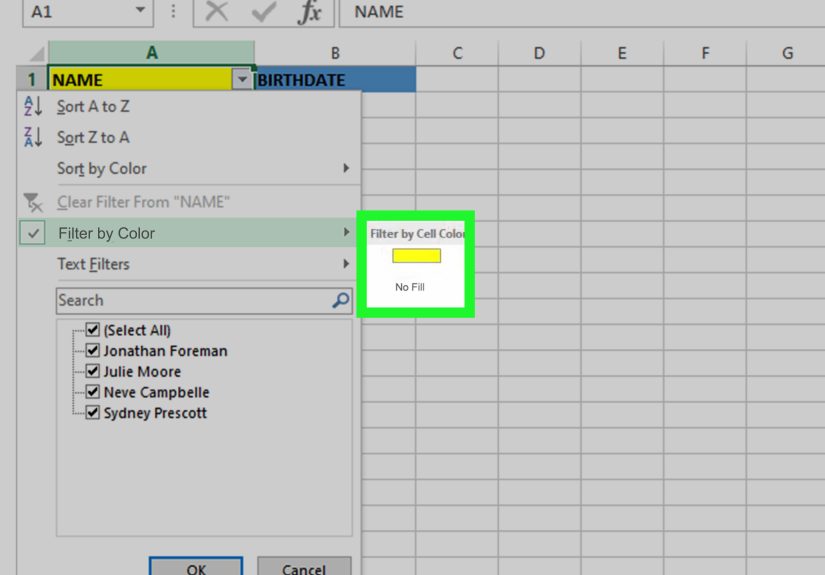
This is the “I just want the yellow-highlighted items” method. Excel’s AutoFilter can filter by fill color in a column.

Step-by-step (Windows desktop Excel)

1. Click anywhere inside your data range (or table).
2. Go to the Data tab on the ribbon.
3. Click Filter. You’ll see small dropdown arrows appear in your header row.
4. Click the dropdown arrow in the column where the color appears.
5. Hover over Filter by Color.
6. Select the color you want (e.g., Yellow under Cell Color).

Result: Excel will show only rows where that column’s cells match your chosen fill color. Everything else is hidden (not deletedExcel is dramatic, not destructive).

Example

Imagine a list of invoices where the “Status” cells are colored:

• Red = Overdue
• Yellow = Needs review
• Green = Paid

Filtering the “Status” column by red fill instantly isolates overdue invoices so you can focus on what matters (and pretend the rest doesn’t exist for five minutes).

Handy shortcut

Turning filters on/off quickly often uses Ctrl + Shift + L in Windows Excel. It’s like flipping the “serious data mode” switch.

Method 2: Filter by Font Color (Because Sometimes the Text Is the Signal)

Filtering by font color works the same way as fill color. This is common when people mark exceptions by turning text red instead of highlighting the cell.

Steps

1. Enable filters (Data > Filter) if you haven’t already.
2. Click the dropdown arrow on the relevant column.
3. Choose Filter by Color.
4. Select the color under Font Color.

Tip: If you don’t see font color options, make sure the colored formatting is in the column you’re filteringnot in some other column of the same row.

Method 3: Filter by Conditional Formatting Icon (Yes, Those Little Arrows Count)

If you use conditional formatting icon sets (like traffic lights, arrows, flags), Excel can filter based on those icons too.

Steps

1. Turn on filters.
2. Click the dropdown arrow in the icon column.
3. Hover over Filter by Color.
4. Select the icon under Cell Icon.

When it’s useful: KPI dashboards, scorecards, and any sheet where icons represent performance tiers.

Method 4: Convert Your Range to a Table (Filtering Gets Friendlier)

Excel tables are like regular ranges that went to finishing school. They come with built-in filtering and make it harder to accidentally filter only half your dataset.

How to do it

1. Click anywhere in your data.
2. Go to Insert > Table.
3. Confirm the range and check My table has headers.
4. Now filter by color using the same dropdown steps as Method 1.

Why this helps: Tables expand automatically as you add rows, and filters behave more predictably when your dataset grows.

How to Clear a Color Filter (So Your Data Comes Back)

Filtering is great until you forget it’s on and panic because “Excel deleted half my rows.” To clear:

• Click the filtered column dropdown and choose Clear Filter From…
• Or go to Data > Clear (clears filters across the sheet)
• Or toggle filters off with Data > Filter again

Common Problems: “Filter by Color” Is Missing or Not Working

If you don’t see Filter by Color or it does nothing, here are the most common causes and fixes.

1) Your data range is broken (blank rows, blank columns, or random islands of data)

Excel decides what “the dataset” is based on contiguous data. Blank rows inside the range can cause the filter to apply incorrectly.

Fix: Remove blank rows within the dataset, or convert the range to a Table so Excel treats it as one unit.

2) Merged cells are interfering

Merged cells often break normal spreadsheet behaviors, including filtering.

Fix: Unmerge cells in the filtered column (and ideally replace merges with “Center Across Selection” formatting if you need the look).

3) You’re using Excel for the web or a shared environment where behavior differs

Some users report cases where filtering by color appears available but doesn’t apply as expected in online scenarios.

Fix: Try opening the file in the desktop app. If it’s a shared workbook setup with feature limitations, consider modern co-authoring instead of legacy sharing.

4) Conditional formatting colors don’t behave like “real” fills in some cases

Filtering by color is based on the visible formatting, but complex conditional formatting setups can create confusionespecially if multiple rules overlap.

Fix: Simplify rules, ensure only one rule determines fill, or consider a helper column approach (below).

Can You Filter by Multiple Colors at Once?

Excel’s built-in Filter by Color typically applies one color at a time per column. If your workflow requires “show red and yellow,” you have a few options:

Option A: Filter one color, copy visible rows, repeat

This is the “manual but fast” method:

1. Filter by Red
2. Select visible rows and copy to a new sheet
3. Clear filter
4. Filter by Yellow
5. Copy visible rows below the red results

It’s not elegant, but neither is your coworker’s habit of coloring entire rows “just in case.”

Option B: Use a helper column to convert color into data

If color represents meaning, the most reliable solution is to store that meaning in a real column (e.g., Status = “Overdue”). Then you filter by the text value, not the paint.

Best practice: Add a “Status” dropdown list (Data Validation) and use conditional formatting to color it. That way, you can filter by the status value and still keep the visual.

Option C: Use VBA or custom functions (advanced users)

If you absolutely must filter by multiple colors programmatically, VBA can do it. This is usually overkill unless you’re repeating the task daily and Excel is basically your second job.

Filter vs. Sort by Color (They’re Not the Same)

Filtering shows only matching rows. Sorting rearranges your data so colors group together.

When to sort by color

• You want to review items in priority order without hiding data
• You want all red items at the top, then yellow, then green

How to sort by color (quick overview)

1. Select your data (or click inside your table)
2. Go to Data > Sort
3. Choose the column
4. Set Sort On to Cell Color (or Font Color / Cell Icon)
5. Pick the color and choose On Top
6. Add levels for additional colors

Pro Tips for Cleaner Color-Based Filtering

Tip 1: Use consistent colors (Excel is literal)

If you use five slightly different shades of yellow, Excel will treat them as five different criteria. Choose one “official” yellow and stick to it. Your future self will thank you.

Tip 2: Color a single column, not random cells everywhere

Filtering by color works per column. If your color markers are scattered across multiple columns, you’ll be forced into awkward multi-step filtering.

Better: Put the “flag color” in one column (like “Status”) and color only that column.

Tip 3: Combine color filtering with SUBTOTAL for quick counts and sums

After filtering by color, you can use SUBTOTAL to calculate totals for visible rows only. This is great for “sum the yellow items” style tasks without manually selecting anything.

Example: If column D contains amounts, use SUBTOTAL(109, D:D) to sum visible cells (109 ignores hidden rows).

Tip 4: Reapply filters after data changes

If your data updates (new rows added, formatting changed), you may need to reapply the filter so Excel refreshes results.

Conclusion

Filtering colored cells in Excel is one of those features that feels like a secret handshake: once you know it exists, you wonder why you ever lived without it. The key is simple:

• Turn on filters (Data > Filter)
• Use the column dropdown
• Choose Filter by Color (cell color, font color, or icon)
• Keep your dataset clean so the feature behaves

And if you find yourself relying on colors for business logic, consider upgrading your process: store meaning in real values (Status, Priority, Category) and let conditional formatting handle the visuals. Excel is happiest when colors are decorationnot the only plan.

Extra: Real-World Experiences Filtering Colored Cells in Excel (500+ Words)

Let’s talk about what actually happens in the wild, where spreadsheets are less “clean dataset” and more “digital junk drawer with formulas.” Filtering by color sounds straightforward until real people start using color like emotional punctuation.

Experience #1: The “Rainbow Status System” That Nobody Documented
I once opened a shared sales tracker where every rep used their own highlight logic. One person used red for “bad lead,” another used red for “call today,” and a third used red because… it matched their brand vibe. Filtering by red produced a list of items that looked urgent, but it was really just a mash-up of three different opinions wearing the same outfit. The fix wasn’t a fancy Excel trickit was a two-minute standard: define what each color means and restrict coloring to one status column. After that, filtering by color actually worked like a tool, not a guessing game.

Experience #2: Conditional Formatting Made the Sheet Look Smart… Until It Didn’t
Another time, a finance sheet used conditional formatting to shade expenses over budget in orange and severe overruns in red. Filtering by color was perfect for quickly pulling “problem items.” But then someone added a new rule on topsomething like “highlight weekends in gray” across the same column. Suddenly, some entries looked gray and red depending on where you clicked, and filtering results felt inconsistent. The lesson: conditional formatting rules can overlap and create unexpected “visual truth.” When the goal is color-based filtering, keep the rule set simple and make sure one rule clearly wins.

Experience #3: The Merged-Cell Trap
If you’ve ever wondered why Excel users speak about merged cells the way campers speak about bearsthis is why. A project schedule had merged cells for phase headers in the same column used for color flags. Filtering by color didn’t behave, and half the team assumed Excel was broken. It wasn’t broken; it was just dealing with merged cells like they’re a prank. Unmerging fixed the filter immediately. Moral of the story: merged cells might look nice, but they come with hidden fees.

Experience #4: “Filter by Color” as a Debugging Tool
A surprisingly great use case: debugging data entry errors. When training a team, we told them to highlight any row they were unsure about in yellow. At review time, the supervisor filtered by yellow and handled only those items. This reduced review time because you weren’t scanning every rowyou were scanning the rows that users already flagged. It’s like crowdsourcing “where I’m not confident” without a complicated workflow.

Experience #5: When Color Is a Shortcut… and When It’s a Crutch
Filtering by color is fantastic for quick triage. But if color is the only way you can identify important rows, you’re one accidental “Format Painter” away from disaster. The most reliable pattern I’ve seen is: store meaning in a column (like Priority = High/Medium/Low), then use conditional formatting to color it. You get the best of both worlds: accurate filtering by value and fast scanning by color.

So yesfiltering colored cells is genuinely useful. Just remember: color is a great assistant, but a terrible manager. Give it a structure to work with, and Excel becomes a lot more predictable (and your spreadsheets become a lot less haunted).